Distance Metrics

This chapter argues that Pearson's correlation is a limited measure of codependence because it is not a true metric, it only captures linear relationships, and it is sensitive to outliers. It introduces concepts from information theory, primarily entropy, as a more robust foundation for measuring distance and similarity, which is critical for many machine learning algorithms.

Correlation-Based Metrics

While correlation ($\rho$) itself is not a distance metric, it can be used to create one. A true metric must satisfy non-negativity and the triangle inequality.

• For Long-Only Portfolios: This metric treats negative correlations as highly distant, which is useful for diversification.
  $$d_{\rho}[X, Y]=\sqrt{\frac{1}{2}(1-\rho[X, Y])}$$
• For Long-Short Portfolios: This metric (a true metric on the $\mathbb{Z} / 2 \mathbb{Z}$ quotient) treats highly positive and highly negative correlations as "close" (i.e., strong relationships).
  $$d_{|\rho|}[X, Y]=\sqrt{1-|\rho[X, Y]|}$$

The text proves these are true metrics by showing they are linear multiples of the Euclidean distance between the z-standardized vectors.

Information Theory Concepts

To overcome the limitations of correlation (linearity, outliers), the chapter introduces entropy-based measures.

• Shannon's Entropy $H[X]$: Measures the amount of uncertainty associated with a random variable $X$. It is maximized when all outcomes are equally probable.
  $$H[X]=-\sum_{x \in S_{X}} p[x] \log [p[x]]$$
• Joint Entropy $H[X, Y]$: Measures the total uncertainty of two variables $X$ and $Y$.
  $$H[X, Y]=-\sum_{x, y \in S_{X} \times S_{Y}} p[x, y] \log [p[x, y]]$$
• Conditional Entropy $H[X \mid Y]$: Measures the remaining uncertainty in $X$ after $Y$ is known.
  $$H[X \mid Y]=H[X, Y]-H[Y]$$
• Kullback-Leibler (KL) Divergence $D_{K L}[p \mid q]$: Measures how much a probability distribution $p$ diverges from a reference distribution $q$. It is not a metric because it is not symmetric ($D_{K L}[p \mid q] \neq D_{K L}[q \mid p]$).
  $$D_{K L}[p \mid q]=\sum_{x \in S_{X}} p[x] \log \left[\frac{p[x]}{q[x]}\right]$$
• Cross-Entropy $H_{C}[p \mid q]$: A popular loss function for classification, it measures the uncertainty of $X$ using an incorrect distribution $q$.
  $$H_{C}[p \mid q]=H[X]+D_{K L}[p \mid q]$$

Information-Based Metrics

From these concepts, we can derive true distance metrics.

• Mutual Information (MI): $I[X, Y]$

  • Concept: Measures the "information gain" about $X$ from knowing $Y$. It is a generalized, non-linear measure of correlation.
  • Equation: $I[X, Y] =H[X]-H[X \mid Y]=H[X]+H[Y]-H[X, Y]$
  • Property: $I[X, Y]$ is not a metric because it fails the triangle inequality.

• Variation of Information (VI): $V I[X, Y]$

  • Concept: This is the chapter's preferred true metric based on information theory. It measures the total uncertainty remaining in $X$ and $Y$ after accounting for the information they share.
  • Equation: $V I[X, Y] =H[X \mid Y]+H[Y \mid X]=H[X]+H[Y]-2 I[X, Y]$
  • Normalized VI (Bounded [0,1]): A normalized version useful for comparing distances.
    $$\widetilde{V I}[X, Y]=\frac{V I[X, Y]}{H[X, Y]}=1-\frac{I[X, Y]}{H[X, Y]}$$

Practical Implementation

Discretization (Binning)

Entropy formulas require discrete variables. To use them on continuous data (like returns), the data must be binned. The choice of binning is critical. The chapter provides an optimal binning formula for joint entropy:

• Optimal Bins:
  $$B_{X}=B_{Y}=\text { round }\left[\frac{1}{\sqrt{2}} \sqrt{1+\sqrt{1+\frac{24 N}{1-\hat{\rho}^{2}}}}\right]$$

Distance Between Partitions

The VI metric can also be used to measure the distance between two different clusterings (partitions), $P$ and $P'$, of the same dataset.

• Equation: $V I\left[P, P^{\prime}\right]=H\left[P \mid P^{\prime}\right]+H\left[P^{\prime} \mid P\right]$

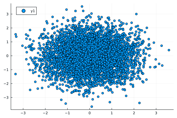
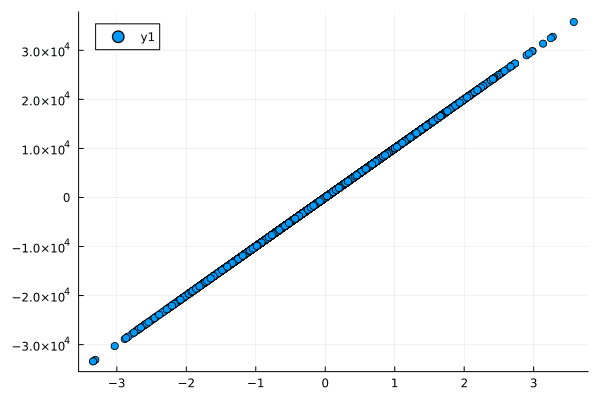
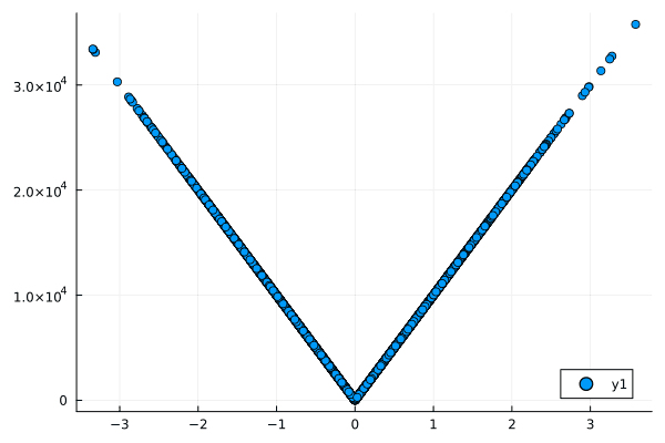
Experimental Results

A test on a nonlinear relationship ($y = |x| + e$) shows that correlation fails ($\rho \approx 0$), while Mutual Information and Variation of Information successfully detect the strong codependence.

Implementation: Information-Theoretic Metrics

To measure the dependence between features, standard linear correlation is often insufficient as it fails to capture non-linear relationships. In the data.distance.distance_metric module, we implement several information-theoretic metrics.

Variation of Information (VI)

The Variation of Information (VI) provides a true metric on the space of partitions. VI(X, Y) = 0 when X and Y are identical, and VI(X, Y) = H(X, Y) when they are independent. We provide a normalized version (by H(X, Y)) to bound the metric between [0, 1].

Mutual Information (MI)

We also implement Mutual Information (MI), which measures the information that X and Y share. We provide a normalized version, MI_norm = MI(X, Y) / min(H(X), H(Y)), which is bounded between [0, 1].

Optimal Binning

Both VI and MI require discretizing the continuous variables. A poor choice of bins can lead to misleading results. We implement a function to calculate the optimal number of bins based on the number of observations and their correlation.

Correlation-Based Distances

Finally, for use in clustering algorithms, we provide functions to convert a correlation matrix into a true distance matrix.

Supported metrics include 'angular' ($\sqrt{0.5 (1 - \rho)}$) and 'absolute_angular' ($\sqrt{0.5 (1 - |\rho|)}$).

API reference

RiskLabAI implements these in Python and Julia (signatures auto-generated from the package source):

def calculate_variation_of_information(
    x: np.ndarray, y: np.ndarray, bins: int, norm: bool = False
) -> float:

function calculate_variation_of_information(
    x::AbstractVector{<:Real},
    y::AbstractVector{<:Real},
    bins::Integer;
    norm::Bool = false,
)

def calculate_number_of_bins(
    num_observations: int, correlation: Optional[float] = None
) -> int:

function calculate_number_of_bins(num_observations::Integer; correlation = nothing)

def calculate_mutual_information(
    x: np.ndarray, y: np.ndarray, norm: bool = False
) -> float:

function calculate_mutual_information(
    x::AbstractVector{<:Real},
    y::AbstractVector{<:Real};
    norm::Bool = false,
)

def calculate_distance(dependence: np.ndarray, metric: str = "angular") -> np.ndarray:

function calculate_distance(
    dependence::AbstractMatrix{<:Real};
    metric::AbstractString = "angular",
)

def calculate_kullback_leibler_divergence(p: np.ndarray, q: np.ndarray) -> float:

function calculate_kullback_leibler_divergence(
    p::AbstractVector{<:Real},
    q::AbstractVector{<:Real},
)

Full source: Python · Julia