Feature Importance

This chapter argues that backtesting is not a research tool; it is a validation step prone to overfitting. The true research tool is feature importance, which helps researchers understand a model's logic, open the "black box," and refine features before running a backtest.

The author establishes a critical maxim:

"Backtesting is not a research tool. Feature importance is."

—Marcos López de Prado

Synthetic Data for Testing

To demonstrate the "substitution effect" and validate the robustness of our feature importance methods, we provide a utility function in features.feature_importance.generate_synthetic_data to generate a complex dataset with a known ground truth.

This function creates a dataset with three types of features:

1. Informative: Features that are truly predictive.
2. Noise: Features that have no predictive value.
3. Redundant: Features that are created by adding noise to the informative features.

This allows us to test if an importance algorithm (like MDI or MDA) correctly identifies the informative features while properly handling (or failing to handle) the redundant and noise features.

The Problem: Substitution Effects

The primary challenge in feature importance is the substitution effect, which is the ML equivalent of multi-collinearity. This occurs when two or more features are correlated (substitutes). Importance algorithms struggle to assign importance correctly, as the features are interchangeable.

• MDI/MDA (explained below) will dilute or incorrectly nullify the importance of these features.
• A partial solution for linear substitution is to first apply Principal Component Analysis (PCA) and run importance tests on the resulting orthogonal features.

Methods (with Substitution Effects)

These methods are standard but are highly vulnerable to substitution effects.

1. Mean Decrease Impurity (MDI)

• Type: In-Sample (IS), fast, and specific to tree-based classifiers (like Random Forests).
• How it Works: MDI measures how much each feature decreases impurity (e.g., Gini, entropy) on average, across all decision tree splits in a forest.
• Key Problems:
  • Substitution: It dilutes importance. If two identical features exist, their importance will be split between them (e.g., 50/50).
  • In-Sample: Being in-sample, even noise features will be assigned some (low) importance.
  • Bias: Can be biased towards features with a large number of categories.

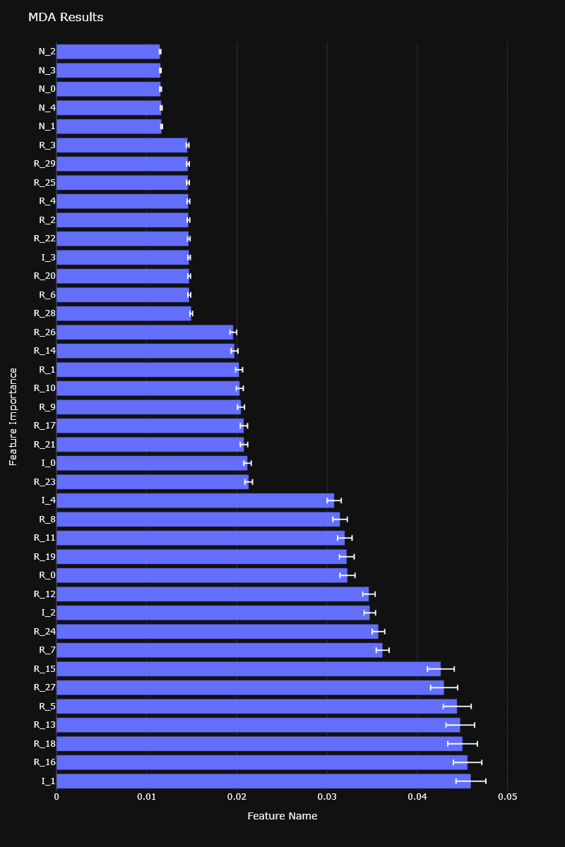
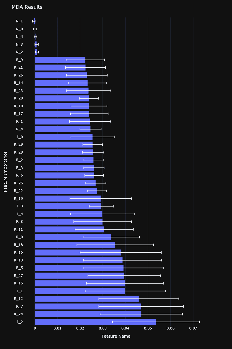
2. Mean Decrease Accuracy (MDA)

• Type: Out-of-Sample (OOS), slow, and works with any classifier.
• How it Works:
  1. A model is trained, and its OOS performance (e.g., accuracy or F1-score) is recorded.
  2. The values for a single feature (one column) are then randomly permuted (shuffled).
  3. The model's OOS performance is re-evaluated on this "corrupted" dataset.
  4. Feature importance is the loss in performance caused by that permutation.
• Key Problems:
  • Substitution: It fails catastrophically. If two features are identical, permuting just one of them has no effect on performance (because the substitute feature is still intact). This causes the algorithm to incorrectly report both features as being completely unimportant.
  • OOS CV: Must be performed using a purged k-fold cross-validation (from Chapter 7) to prevent information leakage.

Methods (without Substitution Effects)

These methods are designed to complement the ones above and mitigate the substitution problem.

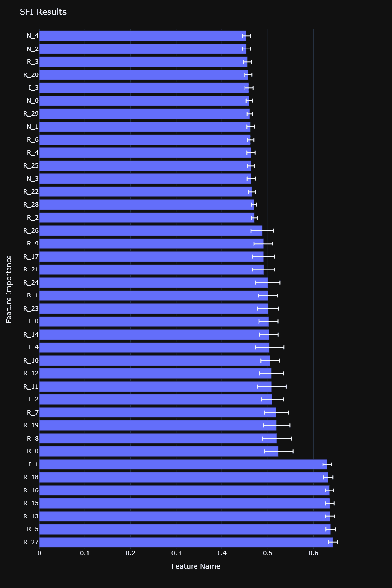
1. Single Feature Importance (SFI)

• Type: Out-of-Sample (OOS).
• How it Works: Instead of a complex model, it tests the OOS performance of a simple classifier built on each feature in isolation.
• Pros: By definition, there are no substitution effects.
• Cons: It misses joint effects. It cannot discover features that are only predictive in combination with other features.

2. Orthogonal Features (using PCA)

This is not a standalone method, but a confirmatory procedure to validate MDI/MDA results and ensure the model is not overfit.

1. Run PCA (Unsupervised): First, run PCA on the features. This ranks features by their variance (eigenvalues) without looking at the labels. This is an "un-overfit" ranking.
2. Run MDI/MDA (Supervised): Run your feature importance method (e.g., MDI) on the new orthogonal features to get a "supervised" ranking.
3. Compare: Calculate the Weighted Kendall's Tau correlation between the PCA rank and the MDI rank.

Key Insight: If the unsupervised PCA ranking and the supervised MDI ranking are highly correlated, it provides strong evidence that the ML model has identified a real, robust pattern and is not just overfit on a statistical fluke.

Research Approaches

• Parallelized: Run feature importance on each instrument (e.g., AAPL, MSFT) separately, then average the results. (Fast, but can be noisy).
• Stacked (Preferred): Stack the data from all instruments into one giant dataset and run the importance analysis once. (Slower, but more robust, general, and less prone to overfitting a single instrument).

Feature Importance Analysis

This chapter argues that feature importance is a critical research tool that is superior to classical methods like p-values. It refutes the "black box" myth of machine learning (ML), showing how ML can be used to understand which variables are important, (the "variable search") before trying to find a specific model (the "specification search").

The Flaws of p-Values

The chapter presents a strong critique of using p-values for feature importance, identifying four key caveats:

1. False Assumptions: p-values rely on strong, often false assumptions about the model specification, regressor correlations, and residual properties.
2. Multicollinearity: They fail in the presence of correlated (redundant) features, leading to "substitution effects" where the importance of related variables cannot be untangled.
3. Wrong Question: A p-value measures P(data | H0) (the probability of the data, given the null hypothesis is true). Researchers actually want P(H0 | data) (the probability the null is true, given the data), which p-values do not provide.
4. In-Sample & p-Hacking: They are an in-sample metric, making them vulnerable to "p-hacking" and false discoveries that do not generalize out-of-sample.

A numerical experiment confirms this, showing that p-values from a logit regression fail to identify most informative features and incorrectly rank noise features as significant.

Machine Learning Alternatives

ML offers robust, non-parametric alternatives that address the flaws of p-values.

Mean-Decrease Impurity (MDI)

• What it is: A fast, in-sample method specific to tree-based models (like Random Forests).
• How it works: It measures a feature's importance by the total reduction in "impurity" (like Gini or entropy) it provides, averaged across all splits in the forest where that feature was used.
• Information Gain Equation:
  $$\Delta g[t, f]=i[t]-\frac{N_{t}^{(0)}}{N_{t}} i\left[t^{(0)}\right]-\frac{N_{t}^{(1)}}{N_{t}} i\left[t^{(1)}\right]$$
• Pros: Solves the first three caveats of p-values (no strong assumptions, robust to substitution via ensembles, answers a relevant question).
• Cons: It is still in-sample (fails caveat 4) and still suffers from substitution effects by diluting the importance of redundant features.

Mean-Decrease Accuracy (MDA)

• What it is: A slower, out-of-sample (OOS) method that works with any model.
• How it works:
  1. The model's OOS performance (e.g., accuracy) is measured using cross-validation.
  2. The values for a single feature column are then randomly shuffled (permuted).
  3. The model's OOS performance is re-measured.
  4. The feature's importance is the drop in performance caused by the shuffling.
• Pros: Solves all four caveats of p-values, especially #4 (it is OOS).
• Cons: Suffers from substitution effects even more severely than MDI. If two features are identical, shuffling one has no effect (as the other is still intact), causing MDA to incorrectly label both as unimportant.

Better Scoring for Financial MDA

The text argues that "accuracy" is a poor metric for MDA in finance because it ignores probabilities (a high-confidence miss is very bad).

• Log-Loss (Cross-Entropy): A better alternative, as it heavily penalizes confident, wrong predictions.
• Probability-Weighted Accuracy (PWA): A proposed alternative that is more intuitive than log-loss. It is an accuracy measure that gives more weight to high-confidence predictions.
  • Equation:
    $$\mathrm{PWA}=\sum_{n=0}^{N-1} y_{n}\left(p_{n}-K^{-1}\right) / \sum_{n=0}^{N-1}\left(p_{n}-K^{-1}\right)$$

The Solution: Clustered Feature Importance (CFI)

CFI is presented as the solution to the substitution effect (multicollinearity) problem that plagues both classical p-values and standard MDI/MDA.

The process has two steps:

1. Cluster Features: First, group all similar (redundant) features together. This can be done using correlation or, more robustly, information-theoretic metrics (like Variation of Information) combined with an optimal clustering algorithm (like ONC).
2. Run Importance on Clusters:
   • Clustered MDI: Instead of getting the importance of individual features, you sum the MDI scores of all features within a cluster to get the cluster's total importance.
   • Clustered MDA: Instead of shuffling one feature at a time, you shuffle all features in a cluster simultaneously. This measures the cluster's true joint importance.

An experiment shows that CFI successfully identifies all 5 informative clusters and correctly assigns near-zero importance to the 1 noise cluster, solving the substitution problem that confused the standard methods.

API reference

RiskLabAI implements these in Python and Julia (signatures auto-generated from the package source):

def orthogonal_features(
    features: pd.DataFrame, variance_threshold: float = 0.95
) -> tuple[pd.DataFrame, pd.DataFrame]:

function orthogonal_features(
    features::AbstractMatrix{<:Real};
    variance_threshold::Real = 0.95,
)

def calculate_weighted_tau(
    feature_importances: np.ndarray, principal_component_ranks: np.ndarray
) -> float:

function calculate_weighted_tau(
    feature_importances::AbstractVector{<:Real},
    principal_component_ranks::AbstractVector{<:Real},
)

class FeatureImportanceMDI(FeatureImportanceStrategy):

function feature_importance_mdi(
    x::AbstractMatrix{<:Real},
    y::AbstractVector;
    n_trees::Integer = 100,
    n_subfeatures::Integer = -1,
    max_depth::Integer = -1,
    random_state::Integer = 0,
)

class FeatureImportanceMDA(FeatureImportanceStrategy):

function feature_importance_mda(
    x::AbstractMatrix{<:Real},
    y::AbstractVector;
    n_splits::Integer = 10,
    n_trees::Integer = 100,
    n_subfeatures::Integer = -1,
    max_depth::Integer = -1,
    random_state::Integer = 42,
)

class FeatureImportanceSFI(FeatureImportanceStrategy):

function feature_importance_sfi(
    x::AbstractMatrix{<:Real},
    y::AbstractVector;
    n_splits::Integer = 10,
    n_trees::Integer = 100,
    max_depth::Integer = -1,
    scoring::Symbol = :log_loss,
    random_state::Integer = 0,
)

def get_test_dataset(
    n_features: int = 100,
    n_informative: int = 25,
    n_redundant: int = 25,
    n_samples: int = 10000,
    random_state: int = 0,
    sigma_std: float = 0.0,
) -> tuple[pd.DataFrame, pd.Series]:

function get_test_dataset(;
    n_features::Integer = 40,
    n_informative::Integer = 10,
    n_redundant::Integer = 10,
    n_samples::Integer = 1000,
    random_state::Integer = 0,
    sigma_std::Real = 0.0,
)

Full source: Python · Julia