Fractional Differentiation and Memory

Traditionally, differentiation to an integer degree is used to make a series stationary. However, fractional differentiation allows the exponent to be a real number. This helps to preserve memory.

The fractional model is mathematically expressed using the backshift operator $B$, and a real number exponent $d$ as:

The series is then a dot product:

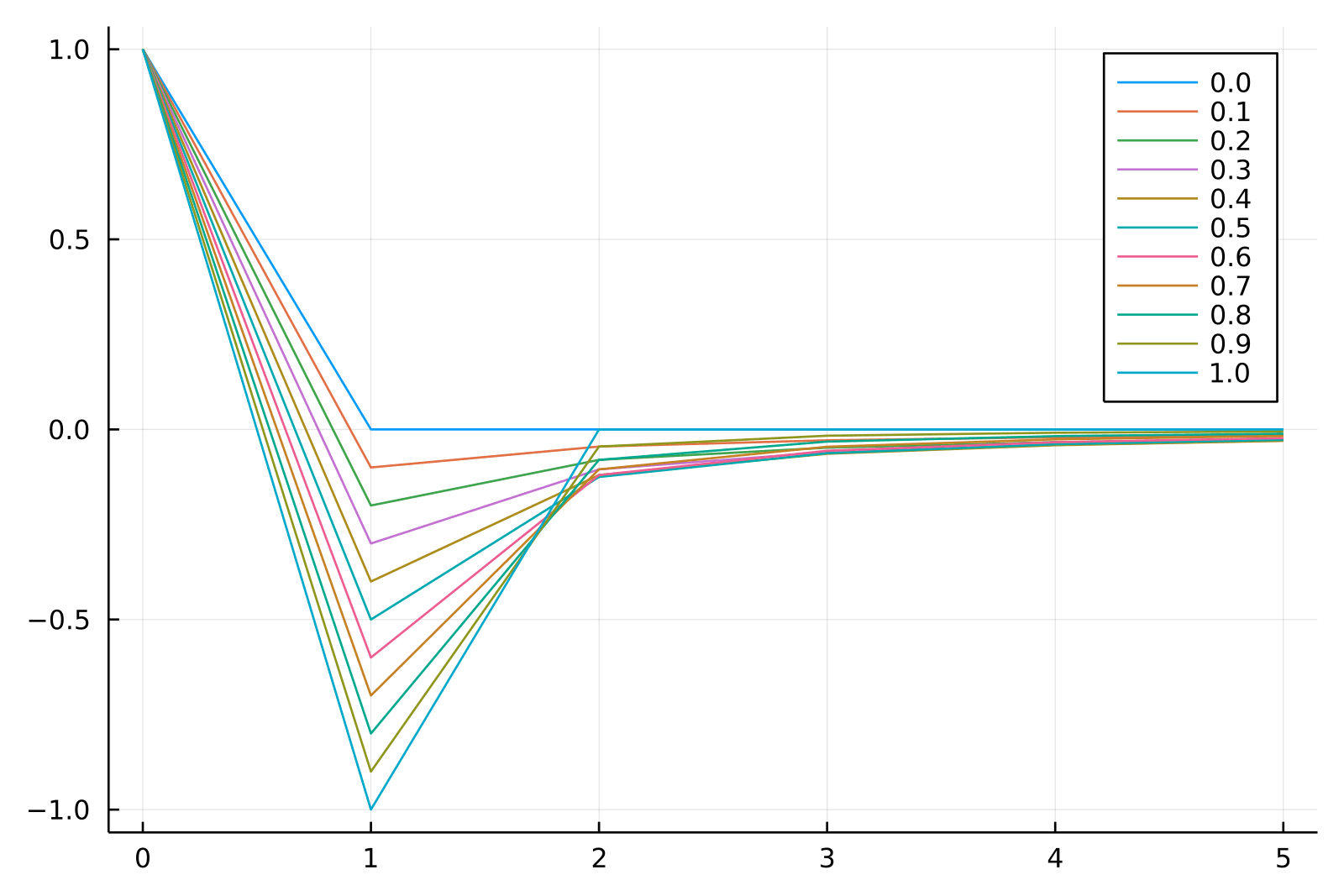
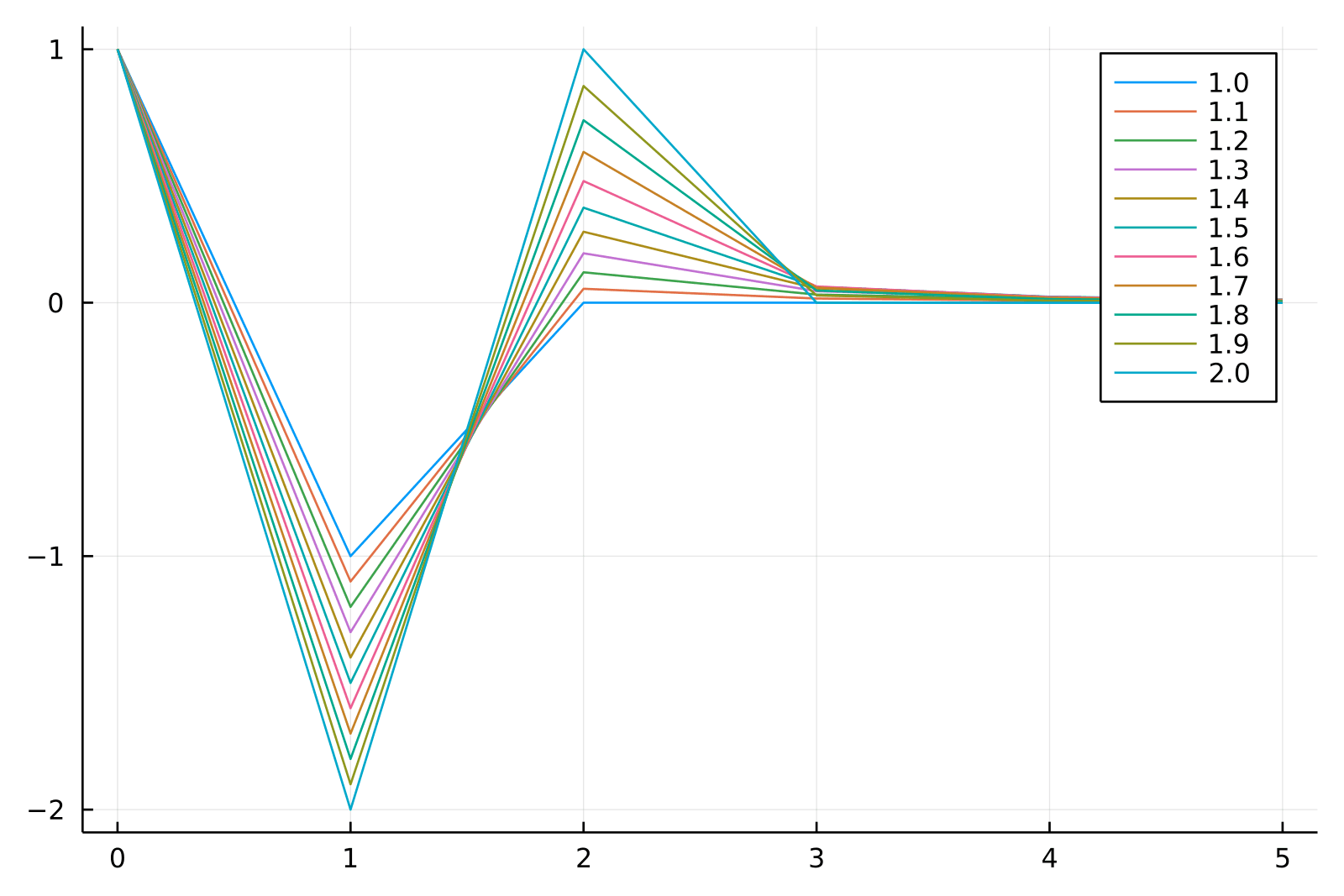
Here, $\omega$ consists of weights calculated based on the degree $d$. The weights alternate in sign and converge to zero as $k$ increases, providing an optimal balance between stationarity and memory.

Weight Sequence and Code Snippets

The sequence of weights can be generated iteratively as:

def weighting(
degree: float,
size: int
) -> list:

def plotWeights(
degreeRange: tuple,
numberDegrees: int,
size: int
) -> None:

function weighting(
degree::Float64,
size::Int
) -> Vector{Float64}

function plotWeights(
degreeRange::Tuple,
numberDegrees::Int,
size::Int
) -> Nothing

View More: Python | Julia

These functionalities are available in both Python and Julia in the RiskLabAI library.

Convergence of Weights

The weights, $\omega$, tend to zero as $k$ increases. Also, the sign of $\omega$ alternates depending on whether $d$ is an integer, even or odd. This property is vital for balancing stationarity and memory in the series.

In summary, fractional differentiation offers a powerful method for transforming non-stationary financial time series into stationary ones while preserving as much memory as possible. This is essential for both inferential statistics and machine learning models in finance.

Fractional Differentiation Methods for Time Series Analysis

In this blog, we'll focus on two techniques for fractional differentiation of a finite time series: the "expanding window" method and the "fixed-width window fracdiff" (FFD) method. These techniques are essential for handling non-stationary time series data in financial analytics.

Expanding Window Method

Given a time series ( { X_t }, t=1, \ldots, T ), this approach involves using varying weights ( \omega_k ) to calculate the fractionally differentiated value $\tilde{X}_T$. The weights depend on the degree of differentiation ( d ) and a tolerance level ( \tau ), which limits the acceptable weight loss for the initial points.

You select a ( l^* ) such that $\lambda_{l^*} \leq \tau$ and $\lambda_{l^*+1} > \tau$. This is to ensure that the weight loss doesn't go beyond a certain threshold.

def fracDiff(series: DataFrame,
degree: float,
threshold: float = 0.01) -> DataFrame:

function fracDiff(series::DataFrame,
degree::Float64,
threshold::Float64 = 0.01) -> DataFrame

View More: Python | Julia

The Fixed-width Window Fracdiff (FFD) method maintains a constant vector of weights $\tilde{\omega}_{k}$ that do not fall below a given threshold ( \tau ).

Thus, the differentiated series $\tilde{X}_t$ is computed as follows:

def fracDiffFixed(series: DataFrame,
degree: float,
threshold: float = 1e-5) -> DataFrame:

function fracDiffFixed(series::DataFrame,
degree::Float64,
threshold::Float64 = 1e-5) -> DataFrame

View More: Python | Julia

Achieving Stationarity

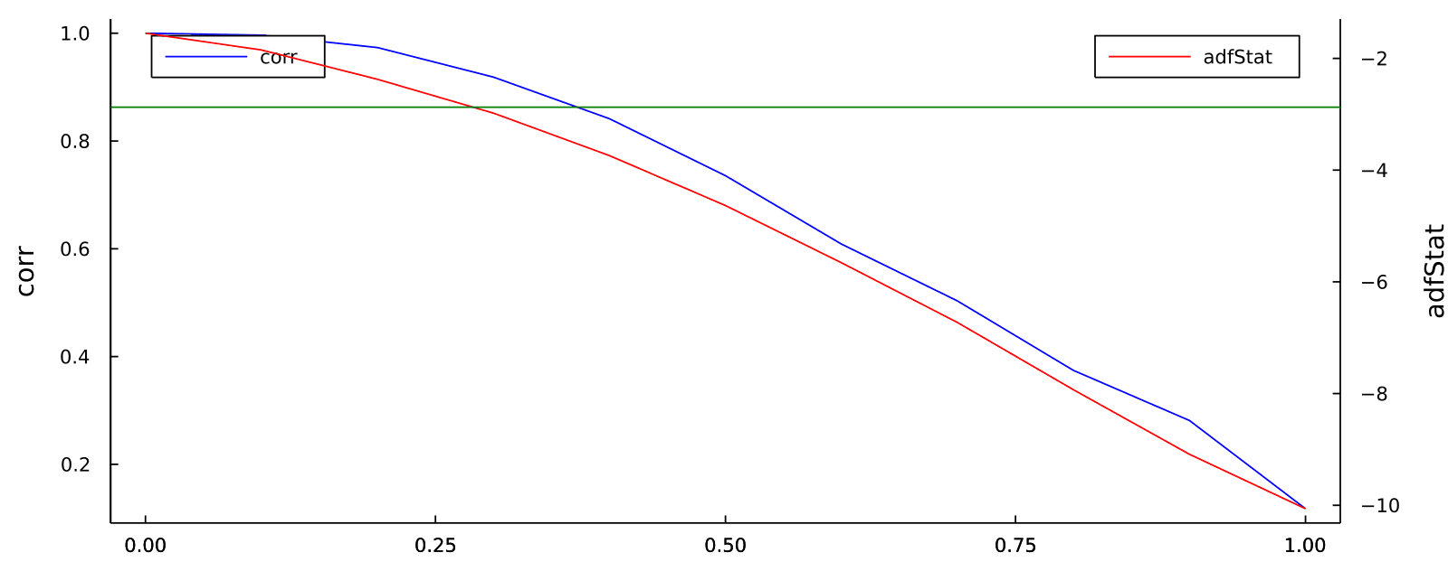
Both methods allow for the quantification of how much memory (or autocorrelation) needs to be removed to achieve a stationary series through the coefficient ( d^* ). Many finance studies have traditionally used integer differentiation, often removing more memory than necessary and potentially losing predictive power.

def minFFD(input: DataFrame) -> float:

function minFFD(input::DataFrame) -> Float64

View More: Python | Julia

References

1. De Prado, M. L. (2018). Advances in financial machine learning. John Wiley & Sons.
2. De Prado, M. M. L. (2020). Machine learning for asset managers. Cambridge University Press.