Financial Data Structures

This document outlines methods for processing and structuring financial data for quantitative analysis, moving from raw data types to structured bars, handling multi-product series, and sampling features for machine learning.

Types of Financial Data

The text identifies four primary types of financial data:

• Fundamental Data: Accounting information that is low-frequency, delayed, and prone to backfilling and forward-looking biases. It is most useful when combined with other data types.
• Market Data: High-frequency trading data (e.g., FIX data) that falls into the "Big Data" category. It can reveal patterns from algorithmic or human trading.
• Analytical Data: Data derived from original sources, often including subjective analysis, which may not be easily replicable.
• Alternative Data: Non-traditional data (e.g., satellite imagery, credit card data) that is difficult to process but can offer a significant predictive edge.

Financial Bars

Bars are used to organize and regularize unstructured, high-frequency market data into a homogeneous format with more favorable statistical properties (e.g., normality, invariance) and reduced noise.

Implementation: Data Structure Controllers

In our RiskLabAI library, we provide a flexible controller system to process raw tick data into various bar types. This system is composed of two main classes:

1. Controller (from data_structure_controller.py): This is the main entry point. It handles reading data efficiently in batches from CSV files or pandas DataFrames and orchestrates the bar construction process.

2. BarsInitializerController (from controller.bars_initializer.py): This class acts as a factory, responsible for creating the specific bar sampling object (e.g., a Dollar Imbalance Bar object) with the correct parameters.

This function takes the method_name (e.g., "expected_dollar_imbalance_bars"), a dictionary of its method_arguments, and the input_data (either a file path or a DataFrame) and processes the data, returning a DataFrame of the constructed bars.

The BarsInitializerController contains static methods for creating each bar type with sensible defaults. Here are some of the key initializers:

• Standard Bars:
• Time Bars:
• Imbalance Bars (Expected vs. Fixed):
• Run Bars (Expected vs. Fixed):

(Note: Implementations for volume_ and tick_ based bars are also available.)

Standard Bars

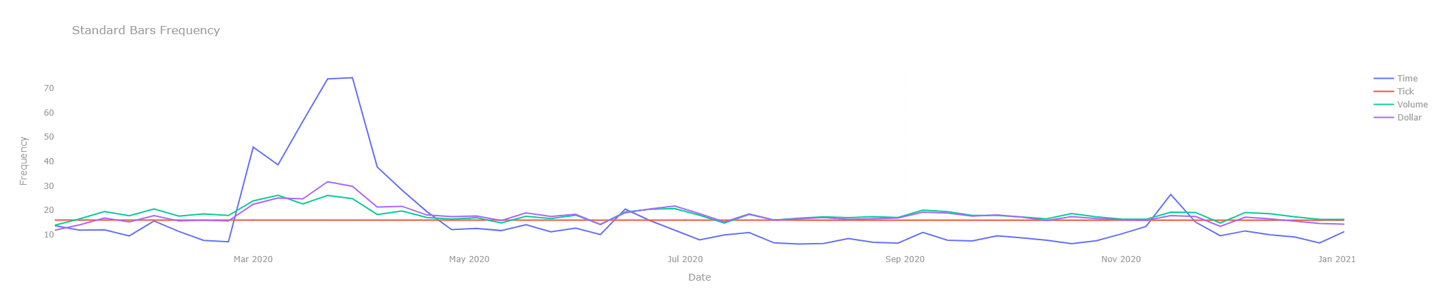
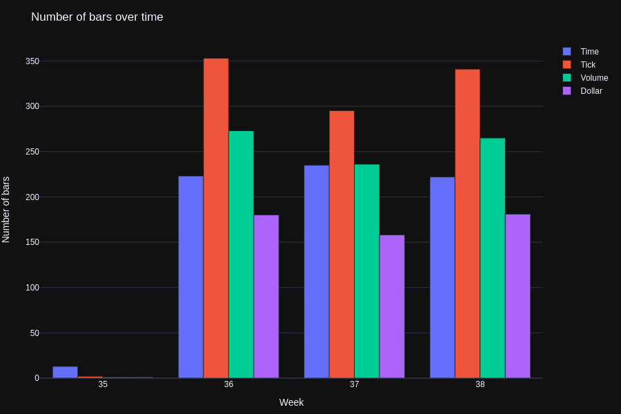
• Time Bars: Data bucketed at regular time intervals (e.g., 1-minute). This method is discouraged as it produces data with unfavorable statistical properties (e.g., heteroscedasticity).
• Tick Bars: Data sampled after a fixed number of trades (ticks). This synchronizes sampling with market activity but is vulnerable to order fragmentation.
• Volume Bars: Data sampled after a fixed number of shares are traded. This resolves the order fragmentation issue seen in tick bars.
• Dollar Bars: Data sampled every time a specific market value (dollar amount) is traded. This is more stable, especially during high turbulence or corporate actions (splits, buybacks) that distort tick and volume counts.

In our RiskLabAI library, we implement the Standard and Time bars, which all inherit from a common AbstractBars class found in RiskLabAI.data.structures.abstract_bars. This base class manages the core logic for bar construction, including the tick rule implementation (_tick_rule), tracking high/low/open/close prices, and formatting the final bar output (_construct_next_bar).

Our implementations for this section are:

1. Time Bars: Implemented in RiskLabAI.data.structures.time_bars as the TimeBars class. This class samples bars based on a fixed time duration, which is configured using a human-readable resolution.

   • resolution_type: A string like 'S', 'MIN', 'H' for seconds, minutes, or hours.
   • resolution_units: An integer for the number of units (e.g., resolution_type='MIN' and resolution_units=5 for 5-minute bars).

2. Standard Bars (Tick, Volume, Dollar): These are implemented in RiskLabAI.data.structures.standard_bars using a single, flexible StandardBars class. The behavior is determined by the bar_type string and a threshold.

   • To create Tick Bars, we set bar_type='CUMULATIVE_TICKS'.
   • To create Volume Bars, we set bar_type='CUMULATIVE_VOLUME'.
   • To create Dollar Bars, we set bar_type='CUMULATIVE_DOLLAR'.

Implementation

In our RiskLabAI library, we provide a utility function in the utilities_lopez module to aggregate tick-level data into standard OHLCV bars. This function efficiently computes the open, high, low, close, total volume, tick count, and VWAP (volume-weighted average price) for each bar.

Information-Driven Bars

These bars sample more frequently when new information is detected in the market, often by tracking imbalances created by informed traders.

1. Tick Imbalance Bars (TIBs) Samples when the cumulative tick imbalance (buy vs. sell ticks) exceeds an expected threshold.

• Tick Direction:
  $$b_{t}= \begin{cases}b_{t-1} & \text { if } \Delta p_{t}=0 \\ \frac{|\Delta p_{t}|}{\Delta p_{t}} & \text { if } \Delta p_{t} \neq 0\end{cases}$$
• Tick Imbalance:
  $$\theta_{T}=\sum_{t=1}^{T} b_{t}$$
• Expected Imbalance:
  $$\mathbb{E}_{0}\left(\theta_{T}\right) = \mathbb{E}_{0}(T)\left(2 \mathrm{P}\left(b_{t}=1\right)-1\right)$$
• Sampling Condition:
  $$T^{\checkmark}=\underset{T}{\arg \min }\left\{|\theta_{T}| \geq \underbrace{\mathbb{E}_{0}(T)|2 \mathrm{P}\left(b_{t}=1\right)-1|}_{|E(\theta_T)|}\right\}$$

2. Volume and Dollar Imbalance Bars (VIBs/DIBs) Extends TIBs by weighting the imbalance by volume or dollar value.

• Imbalance Indicator:
  $$\theta_{T}=\sum_{t=1}^{T} b_{t} v_{t}$$
• Expected Imbalance:
  $$\mathbb{E}_{0}\left(\theta_{T}\right)=\mathbb{E}_{0}(T)\left(2 v^{+}-\mathbb{E}_{0}\left(v_{t}\right)\right)$$
• Sampling Condition:
  $$T^{v}=\underset{T}{\arg \min }\left\{|\theta_{T}| \geq \mathbb{E}_{0}(T)|2 v^{+}-\mathbb{E}_{0}\left(v_{t}\right)|\right\}$$

3. Tick Runs Bars (TRBs) Samples based on consecutive sequences (runs) of buys or sells, which can indicate algorithmic order execution.

• Imbalance Indicator:
  $$\theta_{T}=\max \left\{\sum_{t \mid b_{t}=1}^{T} b_{t},-\sum_{t \mid b_{t}=-1}^{T} b_{t}\right\}$$
• Expected Imbalance:
  $$\mathbb{E}_{0}\left(\theta_{T}\right)=\mathbb{E}_{0}(T) \max \left \{\mathrm{P}\left(b_{t}=1\right), 1-\mathrm{P}\left(b_{t}=1\right)\right\}$$
• Sampling Condition:
  $$T^{\checkmark}=\underset{T}{\argmin}\left \{|\theta_{T}| \geq \underbrace{|\mathbb{E}_{0}(T) \max\left(\mathrm{P}\left(b_{t}=1\right), 1-\mathrm{P}\left(b_{t}=1\right)\right)|}_{|\mathbb{E}_0(\theta_t)|}\right\}$$

4. Volume and Dollar Runs Bars (VRBs/DRBs) Applies the "runs" concept to volume or dollar amounts.

• Imbalance Indicator:
  $$\theta_{T}=\max \left\{\sum_{t \mid b_{t}=1} ^{T} b_{t} v_{t},-\sum_{t \mid b_{t}=-1}^{T} b_{t} v_{t}\right\}$$
• Expected Imbalance:
  $$\mathbb{E}_{0}\left(\theta_{T}\right)=\mathbb{E}_{0}(T) \max \left \{\mathrm{P}\left(b_{t}=1\right) \mathbb{E}_{0}\left(v_{t} \mid b_{t}=1\right), \left(1-\mathrm{P}\left(b_{t}=1\right)\right) \mathbb{E}_{0}\left(v_{t} \mid b_{t}=-1\right)\right\}$$
• Sampling Condition:
  $$T^{\checkmark} = \underset{T}{\arg \min }\left \{\theta_{T} \geq \underbrace{\mathbb{E}_{0}(T) \max{\Big(...\Big)}}_{|\mathbb{E}_0(\theta_t)|}\right\}$$

Dealing with Multi-Product Series

This section covers methods for modeling a basket of securities (like a spread or portfolio) as a single time series.

• The ETF Trick: A method to convert a multi-product dataset (e.g., a futures spread) with dynamic weights into a single, continuous total-return series, similar to an ETF. It accounts for holdings, PnL, dividends, and transaction costs.
  • Holdings:
    $$h_{i, t}=\left\{\begin{array}{cc} \frac{\omega_{i, t} K_{t}} {o_{i, t+1} \varphi_{i, t} \sum_{i=1}^{I}|\omega_{i, t}|} & \text { if } t \in B \\ h_{i, t-1} & \text { otherwise } \end{array}\right.$$
  • Investment Value:
    $$K_{t}=K_{t-1}+\sum_{i=1}^{I} h_{i, t-1} \varphi_{i, t}\left( \text{PnL}_{i, t}+d_{i, t}\right)$$
  • Tradeable Basket Units (Volume):
    $$v_{t}=\min _{i}\left\{\frac{v_{i, t}}{| h_{i, t-1}|}\right\}$$
• PCA Weights: A method to determine portfolio weights ($\omega$) that achieve a user-defined risk distribution ($R$) across the principal components (eigenvectors) of the covariance matrix ($\Sigma$).
  • Covariance Decomposition: $\Sigma =P \Lambda P'$
  • Portfolio Risk: $\sigma^{2}=\omega^{\prime}\Sigma\omega = \sum_{n=1}^{N} (\omega_\bot)_{n}^{2} \Lambda_{n, n}$
  • Risk per Component: $R_{n}=(\omega_\bot)_{n}^{2} \Lambda_{n, n} \sigma^{-2}$
  • Allocation (Orthogonal Basis): $\omega_\bot=\left\{\sigma \sqrt{\frac{R_{n}}{\Lambda_{n, n}}}\right\}_{n=1, \ldots, N}$
  • Allocation (Original Basis): $\omega=W \omega_\bot$
• Single Future Roll: A method to create a continuous futures series by calculating and subtracting the cumulative "roll gaps." A more robust method for generating non-negative prices is to compute returns using the rolled price change divided by the raw price, and then take a cumulative product of (1+r).

In our RiskLabAI.asset_allocation.hedging module, we implement this PCA-based weighting method with the pca_weights function.

This function calculates the eigenvalues and eigenvectors of the covariance matrix. As described in the methodology, a user can pass a specific risk_distribution (the $R$ vector) to define the target risk allocation across the principal components, and a risk_target (the $\sigma$ value) to scale the overall portfolio. If no risk_distribution is given, the function defaults to allocating 100% of the risk to the component with the smallest eigenvalue, effectively creating a minimum variance portfolio.

Sampling Features

This section discusses methods for selecting relevant observations from structured bars to create feature matrices for ML algorithms.

• Sampling for Reduction:
  • Linspace Sampling: Simple sequential sampling (downsampling).
  • Uniform Sampling: Randomly drawing samples. Both methods are criticized for not necessarily selecting the most informative observations.
• Event-Based Sampling: The preferred method. Samples are "triggered" when a significant event occurs (e.g., volatility spike, structural break), allowing the ML algorithm to learn from relevant market conditions.
• The CUSUM Filter: A specific event-based sampling technique. It detects a shift in the mean of a series. A sample (event) is triggered when the cumulative sum of deviations ($S_t$) from a target value exceeds a threshold $h$.
  • Symmetric CUSUM:
    $$S_{t}^{+}=\max \left\{0, S_{t-1}^{+}+y_{t}-\mathbb{E}_{t-1}\left(y_{t}\right)\right\}, S_{0}^{+}=0$$
    $$S_{t}^{-}=\min \left\{0, S_{t-1}^{-}+y_{t}-\mathbb{E}_{t-1}\left(y_{t}\right)\right\}, S_{0}^{-}=0$$
    $$S_{t}=\max \left\{S_{t}^{+},-S_{t}^{-}\right\}$$
  • Sampling: A bar $t$ is sampled if $S_t \geq h$, at which point the sum $S_t$ is reset. This prevents multiple triggers from small oscillations around the threshold.

API reference

RiskLabAI implements these in Python and Julia (signatures auto-generated from the package source):

class AbstractBars(ABC):

function AbstractBars(bar_type::String)::NamedTuple

class TimeBars(AbstractBars):

function TimeBars(; resolution_type::String, resolution_units::Int)

Full source: Python · Julia