Solving High-Dimensional PDEs with Deep BSDE Methods

High-dimensional parabolic equations are difficult to solve on a full spatial grid. Deep BSDE methods simulate forward paths and learn the value and gradient needed to match a terminal condition.

The central relation

The class of equations studied in the notebooks has the form

\partial_tu+\mu^{\mathsf T}\nabla_xu +\frac12\operatorname{tr}\!\left(\sigma\sigma^{\mathsf T}\nabla_x^2u\right) +f\!\left(t,x,u,\sigma^{\mathsf T}\nabla_xu\right)=0, \qquad u(T,x)=g(x).

$u(t,x)$ is the unknown value, $\mu$ and $\sigma$ are drift and diffusion, and $\nabla_xu$ and $\nabla_x^2u$ are its gradient and Hessian. The driver is $f$ , the terminal value is $g$ , and $T$ is the final time.

Learning PDE solutions from simulated paths

The path plot shows the simulated states that drive training. The benchmark comparison reports relative error across several equations and dimensions.

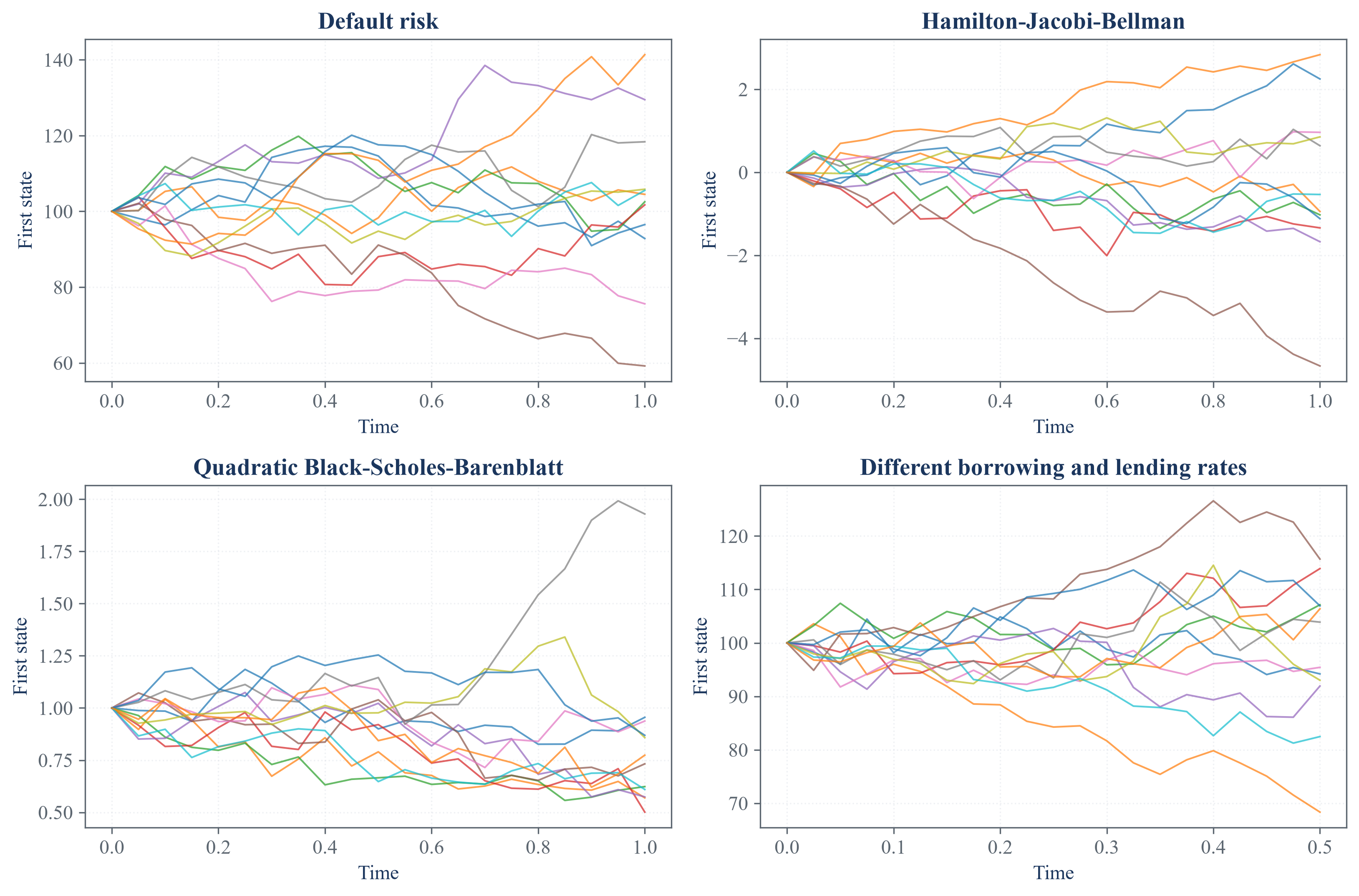
Simulated forward state paths used by a deep BSDE solver. — The solver trains on sampled paths rather than a full spatial grid. Each path carries the state from its initial value to the terminal condition.

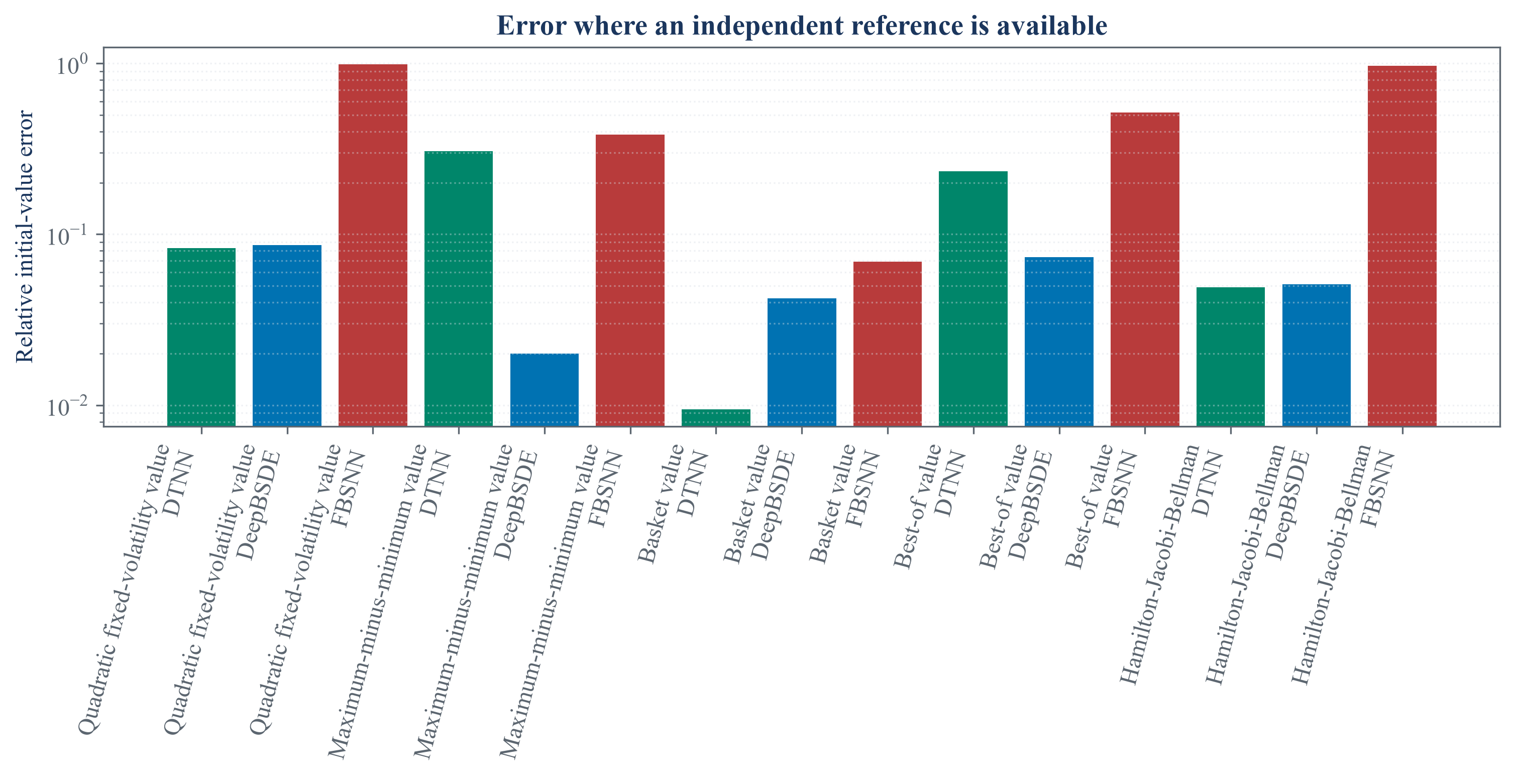
Relative errors for deep BSDE benchmark equations and dimensions. — The benchmark panel compares learned values with available reference solutions, keeping numerical error visible beside training loss.

A low training loss is not itself a solution guarantee. Reference values, repeated seeds, time-step checks, and dimension checks remain necessary.

Notebooks


1. From parabolic equations to backward stochastic representations
2. Training a neural solver on simulated paths
3. Benchmarking financial equations