The Mathematical Language of Financial Learning

A financial model needs a precise rule for what may be known at each date. These notebooks connect that rule to statistical targets, estimates, decisions, and the uncertainty that remains in a finite sample.

The central relation

An information sequence is written as

(\Omega,\mathcal F,\mathbb P),\qquad \mathcal F_0\subseteq\mathcal F_1\subseteq\cdots\subseteq\mathcal F_T, \qquad R_t\in\mathcal F_t.

$\Omega$ is the set of possible outcomes, $\mathcal F$ is the collection of events, and $\mathbb P$ assigns probabilities. The set $\mathcal F_t$ contains the information available by time $t$ , while $R_t\in\mathcal F_t$ says that the return at time $t$ is known then. The final date is $T$ .

What growing information sets reveal about uncertainty

The experiments make the information sequence visible and then show how a sample estimate behaves as more observations become available.

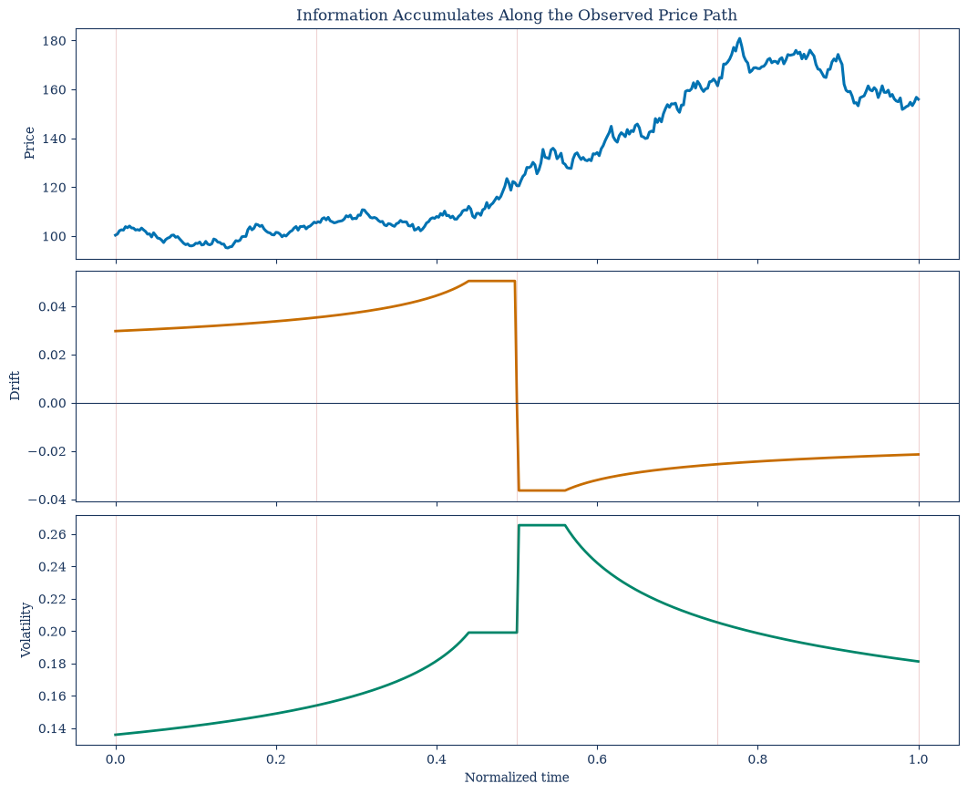
A sequence of nested information sets with returns and innovations arriving through time. — The filtration diagram records when returns and new information enter the model. A decision at a given date may use the current set and its history, but not later observations.

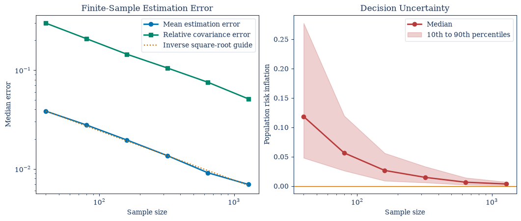
Repeated estimates approaching a known population value as sample size increases. — Repeated samples show the spread of an estimator at several sample sizes. The spread narrows with more observations, while individual estimates still differ from the known target.

The numerical experiment separates an estimand from an estimator: one is the quantity of interest, and the other is a sample-based attempt to learn it.

Notebooks


1. Modeling Financial Information over Time
2. From Statistical Targets to Financial Decisions
3. Measuring Uncertainty in Finite Samples