Portfolio Geometry under Covariance Uncertainty

Mean-variance portfolios are geometric objects built from expected returns, covariance, and constraints. The notebooks show that small estimation changes can move the optimizer sharply, especially near poorly conditioned directions.

The central relation

For portfolio weights $w$ , expected return and variance are

\mu_p=w^{\mathsf T}\mu,\qquad \sigma_p^2=w^{\mathsf T}\Sigma w,\qquad \mathbf 1^{\mathsf T}w=1.

$\mu$ is the asset expected-return vector, $\Sigma$ is the covariance matrix, and $\mu_p$ and $\sigma_p^2$ are portfolio expected return and variance. The last equality requires the weights to sum to one.

How estimation error moves the optimal portfolio

The frontier displays feasible return-risk combinations. The sensitivity plot then changes the estimated mean and covariance inputs and records the resulting portfolio movement.

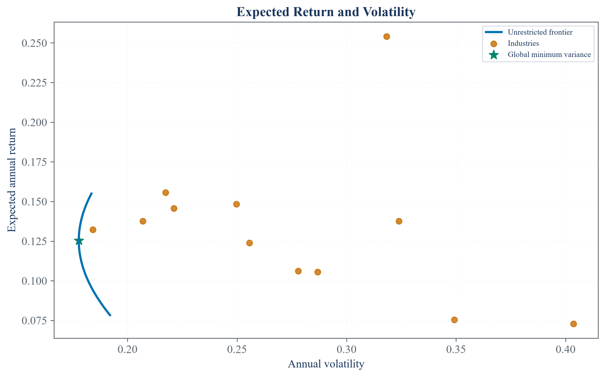
A mean-variance frontier with feasible portfolios and selected constrained solutions. — The frontier traces the smallest variance available for each target return under the stated constraints and estimated inputs.

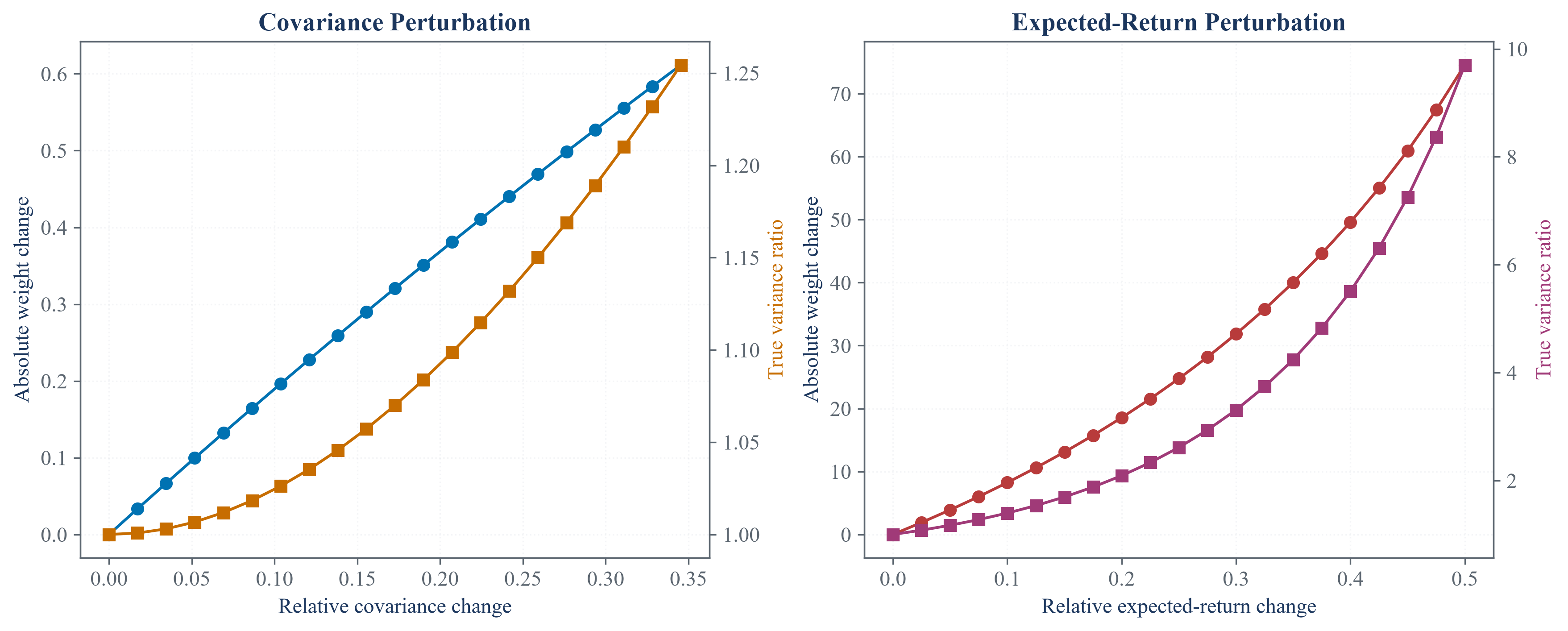
Portfolio-weight and risk sensitivity to changes in mean and covariance estimates. — Input perturbations reveal which portfolio features are stable and which are amplified by the optimization.

An optimizer solves the supplied problem. It does not establish that the estimated inputs are accurate or that the chosen constraints express the right decision.

Notebooks


1. Solving constrained mean-variance portfolios
2. Measuring portfolio sensitivity to estimation error
3. Stress-testing benchmark portfolios