Causal Effects with Network Interference

Many financial and economic actions spread through relationships among units. These notebooks replace the usual no-interference assumption with an exposure rule that records both a unit's own assignment and the assignments of its neighbors.

The central relation

For exposure state $d$ , a Horvitz--Thompson mean is

\widehat\mu(d)=\frac{1}{N}\sum_{i=1}^{N} \frac{\mathbf 1\{D_i=d\}Y_i}{\pi_i(d)}, \qquad \widehat\tau=\widehat\mu(1)-\widehat\mu(0).

$N$ is the number of units, $D_i$ is the exposure state of unit $i$ , $Y_i$ is its observed outcome, and $\pi_i(d)$ is the probability that it receives exposure $d$ . The indicator selects units in that exposure state. The contrast $\widehat\tau$ compares two exposure means.

Estimating spillovers under unequal exposure

The topology figure turns public market associations into an illustrative network. The repeated assignment experiment then checks the weighted estimator against a known contrast under the declared exposure rule.

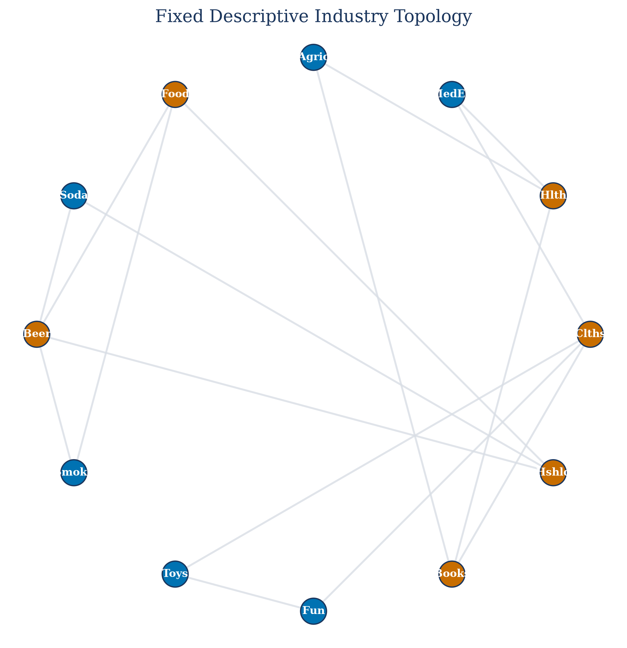
An illustrative network built from public market associations. — The network supplies a visible neighborhood structure for the experiment. Its links describe selected public associations and are not presented as causal relations.

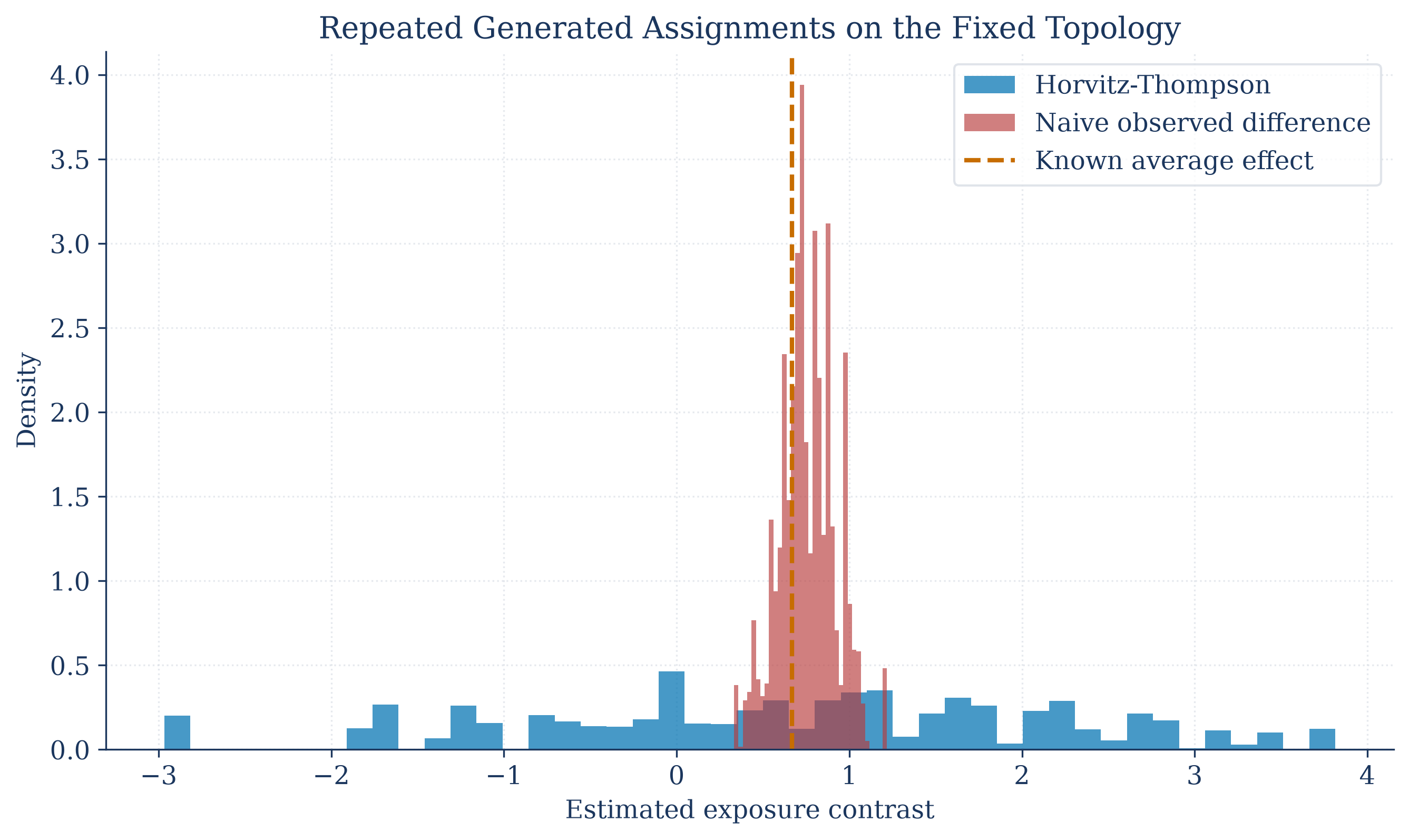
Repeated network exposure estimates compared with a known reference contrast. — Repeated assignments show the sampling variation created by unequal exposure probabilities and the correction supplied by inverse-probability weighting.

The exposure rule and assignment mechanism are part of the causal question. A descriptive correlation network alone does not identify spillover effects.

Notebooks


1. Mapping assignments to network exposure
2. Horvitz-Thompson Exposure Contrasts
3. Where interference estimates remain credible