Generative Models for Financial Time Series

A time-series generator must reproduce more than a one-period distribution. It must also respect chronology and the way the next observation depends on earlier ones. The notebooks prepare ordered windows, train TimeGAN, and examine held-out diagnostics.

The central relation

The joint law of an ordered sequence can be factored as

p(x_{1:T})=p(x_1)\prod_{t=2}^{T}p(x_t\mid x_{1:t-1}).

$x_t$ is the observation at time $t$ , $x_{1:t-1}$ is its preceding history, and $p(x_{1:T})$ is the joint law of the whole sequence. Each conditional factor describes the next observation given what came before it.

Testing realism in generated financial sequences

One figure shows how the TimeGAN components divide the learning task. The other compares real and generated sequences on data not used to fit the model.

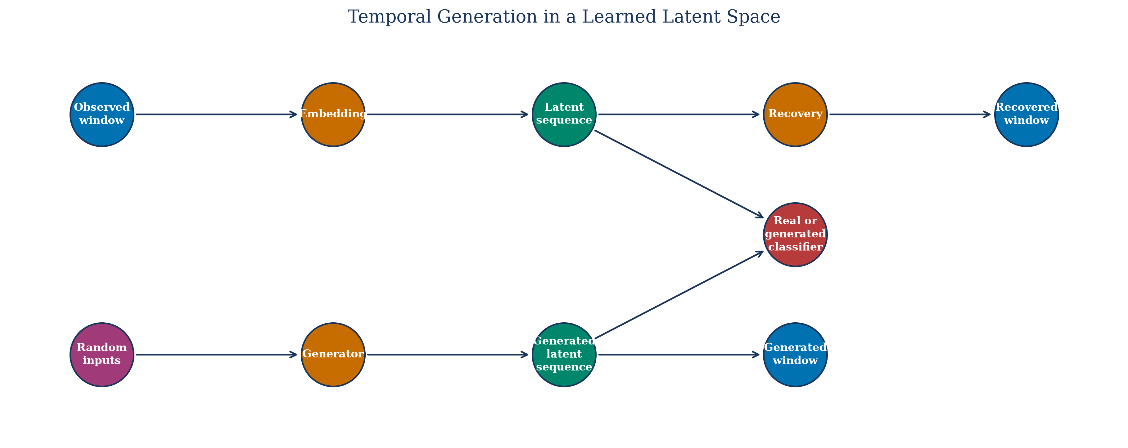
A map of the TimeGAN embedding, recovery, generator, supervisor, and discriminator components. — The component map separates reconstruction, supervised temporal learning, and adversarial discrimination. Each loss checks a different part of the sequence model.

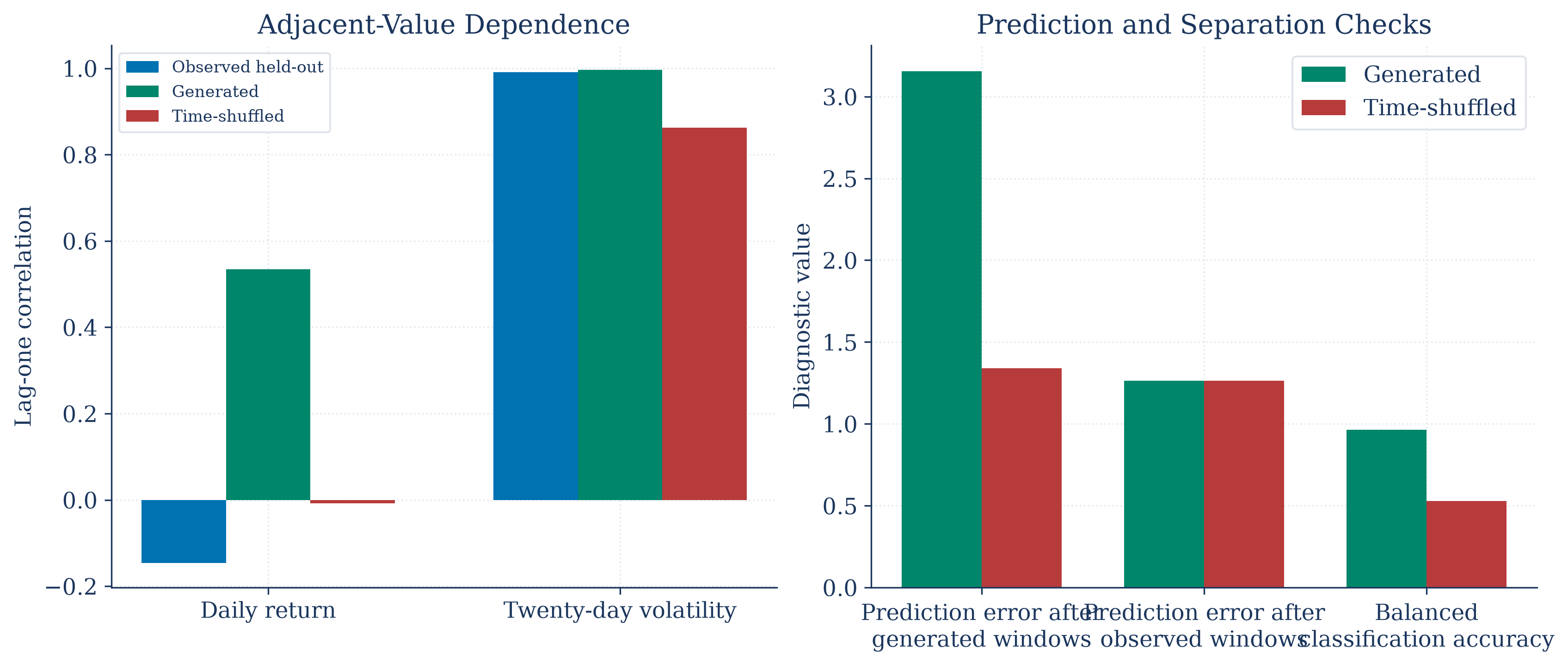
Held-out diagnostic comparisons between real and TimeGAN-generated financial sequences. — Held-out diagnostics compare selected distributional and temporal summaries of real and generated windows. Agreement on these summaries is evidence about those checks only.

A generator may pass several diagnostics and still miss features that were not measured. The notebooks therefore report separate checks rather than one claim of realism.

Notebooks


1. Learning from chronological sequence data
2. Combining adversarial training with temporal structure
3. What held-out diagnostics can establish